
Linear Programming – From Definitions to Complete PYQ Solutions
Linear Programming is a systematic method of finding the maximum or minimum value of a quantity while
following certain conditions. It appears every year in WBCHSE Class 12 exams, and understanding its basic
terms makes the entire chapter far easier to master. Before you dive into the questions, it helps to have
a clear picture of all the essential definitions — just the way textbooks explain them.
This post gives you a concise set of all important terms used in Linear Programming, followed by a complete
collection of solved WBCHSE Class 12 Previous Year Questions from 2015 to 2025. Each problem is presented
with graphs, feasible regions, corner points, and final values of Z so that you can revise the chapter
thoroughly in one place.
Important Definitions
Linear Programming: A mathematical technique used to determine the optimal value (maximum or minimum) of a linear objective function subject to a set of linear constraints.
Objective Function: The function to be optimized, usually written as Z = ax + by.
Decision Variables: The unknown quantities (like x and y) whose values need to be determined in order to optimize Z.
Constraints: The conditions or restrictions on the variables, written in the form of linear inequalities.
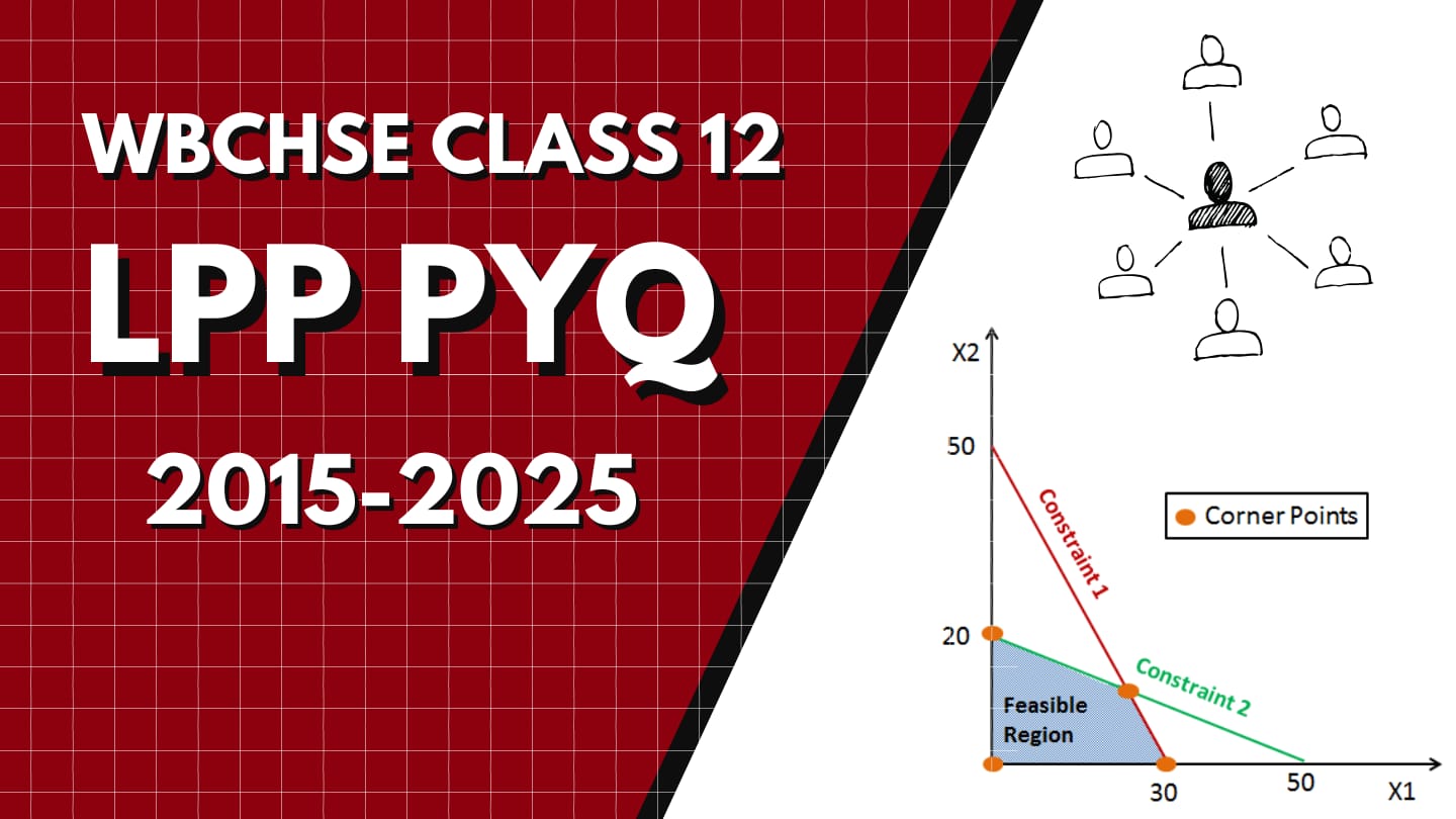
Feasible Region: The region on the graph that satisfies all the constraints simultaneously. Every valid solution lies within this region.
Feasible Solution: Any point within or on the boundary of the feasible region.
Corner Points (Vertices): The intersection points of the boundary lines of the feasible region. The optimal solution always lies at one of these points.
Optimal Solution: The point in the feasible region where the objective function reaches its maximum or minimum value.
Unbounded Solution: When the feasible region extends infinitely and the objective function can increase or decrease without limit.
Infeasible Solution: When no common feasible region exists because the constraints contradict each other.
With these definitions in place, the upcoming section covers all Linear Programming PYQs of WBCHSE Class 12
from 2015 to 2025 — solved step by step with graphs and explanations to strengthen your understanding.
Q1.
MinimizationYear: 2025
Minimize Z = 2x − y Subject to x + y ≤ 5 x + 2y ≤ 8 4x + 3y ≥ 12 x, y ≥ 0
Solution:
1. Reduce to equations: x + y = 5, x + 2y = 8, 4x + 3y = 12. 2. Draw these three lines with the axes in the first quadrant. 3. Check (0, 0): it satisfies x + y ≤ 5 and x + 2y ≤ 8, but not 4x + 3y ≥ 12, so for 4x + 3y ≥ 12 we take the side opposite to (0, 0). 4. The common region with x ≥ 0, y ≥ 0 is the feasible region; its vertices are (0, 4), (2, 3), (5, 0), (3, 0). 5. Compute Z = 2x − y at each vertex to get the minimum value.
Feasible region: bounded; vertices (0, 4), (2, 3), (5, 0), (3, 0).
Graph:
Z = 2x − y at corner points:
| (x, y) | Z |
|---|---|
| (0, 4) | −4 |
| (2, 3) | 1 |
| (5, 0) | 10 |
| (3, 0) | 6 |
∴ Zmin = −4 at (0, 4).
Q2.
MaximizationYear: 2024
Solve the following linear programming problem graphically. Maximize Z = 4x + 3y Subject to x + y ≤ 50 x + 2y ≤ 80 2x + y ≥ 20 x ≥ 0, y ≥ 0
Solution:
1. Boundary equations: x + y = 50, x + 2y = 80, 2x + y = 20. 2. Draw these lines and the coordinate axes in the first quadrant. 3. Check (0, 0): it satisfies x + y ≤ 50 and x + 2y ≤ 80 but not 2x + y ≥ 20, so the feasible side of 2x + y ≥ 20 is away from (0, 0). 4. Intersection of all half-planes with x ≥ 0, y ≥ 0 gives a bounded feasible region with vertices (0, 20), (0, 40), (20, 30), (50, 0), (10, 0). 5. Find Z = 4x + 3y at each vertex and pick the largest value.
Feasible region: bounded; vertices (0, 20), (0, 40), (20, 30), (50, 0), (10, 0).
Graph:
Z = 4x + 3y at corner points:
| (x, y) | Z |
|---|---|
| (0, 20) | 60 |
| (0, 40) | 120 |
| (20, 30) | 170 |
| (50, 0) | 200 |
| (10, 0) | 40 |
∴ Zmax = 200 at (50, 0).
Q3.
MinimizationYear: 2023
Solve the following linear programming problem graphically. Minimize Z = 200x + 500y Subject to the constraints x + 2y ≥ 10 3x + 4y ≤ 24 x ≥ 0, y ≥ 0
Solution:
1. Boundary equations: x + 2y = 10 and 3x + 4y = 24. 2. Draw both lines and the axes in the first quadrant. 3. Check (0, 0): it does not satisfy x + 2y ≥ 10 but satisfies 3x + 4y ≤ 24. 4. Taking correct half-planes, the feasible region (near these lines) has vertices (0, 5), (0, 6) and (4, 3). 5. Evaluate Z = 200x + 500y at these vertices and choose the least value.
Feasible region: effectively bounded; vertices (0, 5), (0, 6), (4, 3).
Graph:
Z = 200x + 500y at corner points:
| (x, y) | Z |
|---|---|
| (0, 5) | 2500 |
| (0, 6) | 3000 |
| (4, 3) | 2300 |
∴ Zmin = 2300 at (4, 3).
Q4.
MaximizationYear: 2022
Solve the linear programming problem graphically. Maximise Z = 4x + y where x + y ≤ 50 3x + y ≤ 90 x ≥ 0 and y ≥ 0
Solution:
1. Boundary equations: x + y = 50 and 3x + y = 90. 2. Draw both lines along with the coordinate axes. 3. Check (0, 0): it satisfies both inequalities, so feasible side for each is towards (0, 0). 4. With x ≥ 0, y ≥ 0, feasible region is a quadrilateral with vertices (0, 0), (0, 50), (20, 30), (30, 0). 5. Compute Z = 4x + y at these vertices and choose the largest value.
Feasible region: bounded; vertices (0, 0), (0, 50), (20, 30), (30, 0).
Graph:
Z = 4x + y at corner points:
| (x, y) | Z |
|---|---|
| (0, 0) | 0 |
| (0, 50) | 50 |
| (20, 30) | 110 |
| (30, 0) | 120 |
∴ Zmax = 120 at (30, 0).
Q5.
MinimizationYear: 2020
Solve the following linear programming problem graphically. Minimize Z = 4x + y Subject to the constraints x + y ≤ 50 3x + y ≤ 90 and x ≥ 0, y ≥ 0
Solution:
1. Constraints are same as Q4, hence vertices of feasible region are (0, 0), (0, 50), (20, 30), (30, 0). 2. Evaluate Z = 4x + y at each of these points. 3. Smallest value is the required minimum.
Feasible region: bounded; vertices (0, 0), (0, 50), (20, 30), (30, 0).
Graph:
Z = 4x + y at corner points:
| (x, y) | Z |
|---|---|
| (0, 0) | 0 |
| (0, 50) | 50 |
| (20, 30) | 110 |
| (30, 0) | 120 |
∴ Zmin = 0 at (0, 0).
Q6.
MinimizationYear: 2019
Solve the following linear programming problem graphically. Minimize Z = 200x + 500y Subject to the constraints x + 2y ≥ 10 3x + 4y ≤ 24 x ≥ 0, y ≥ 0
Solution:
1. Lines are x + 2y = 10 and 3x + 4y = 24 (same as Q3). 2. Draw both lines and axes, then use (0, 0) to decide half-planes. 3. Feasible region for minimum again has vertices (0, 5), (0, 6), (4, 3). 4. Evaluate Z = 200x + 500y at these points and choose the least.
Feasible region: effectively bounded; vertices (0, 5), (0, 6), (4, 3).
Graph:
Z = 200x + 500y at corner points:
| (x, y) | Z |
|---|---|
| (0, 5) | 2500 |
| (0, 6) | 3000 |
| (4, 3) | 2300 |
∴ Zmin = 2300 at (4, 3).
Q7.
MinimizationYear: 2018
Solve the following linear programming problem by graphical method and find the minimum value of Z. Z = 6x + 10y Subject to the constraints x + 2y ≥ 10 2x + 2y ≥ 12 3x + y ≥ 8 x, y ≥ 0
Solution:
1. Boundary equations: x + 2y = 10, x + y = 6, 3x + y = 8. 2. Draw the three straight lines with axes. 3. Origin (0, 0) does not satisfy any ≥ inequality, so feasible region is away from (0, 0) and unbounded. 4. Important corner points near origin are (0, 8), (1, 5), (2, 4). 5. Compute Z = 6x + 10y at these points and take the smallest value.
Feasible region: unbounded; key points (0, 8), (1, 5), (2, 4).
Graph:
Z = 6x + 10y at corner points:
| (x, y) | Z |
|---|---|
| (0, 8) | 80 |
| (1, 5) | 56 |
| (2, 4) | 52 |
∴ Zmin = 52 at (2, 4).
Q8.
MaximizationYear: 2017
Solve the following linear programming problem in graphical method and find the maximum value of Z. Z = x + y Subject to the constraints 5x + 10y ≤ 50 x + y ≥ 1 y ≤ 4 and x, y ≥ 0
Solution:
1. From 5x + 10y ≤ 50 we get x + 2y ≤ 10; equations are x + 2y = 10, x + y = 1, y = 4. 2. Draw these three lines and the axes. 3. Check (0, 0): it satisfies x + 2y ≤ 10 and y ≤ 4, but not x + y ≥ 1, so the feasible side for x + y ≥ 1 is away from (0, 0). 4. The resulting feasible region in first quadrant is a pentagon with vertices (0, 1), (1, 0), (10, 0), (2, 4), (0, 4). 5. Evaluate Z = x + y at each vertex to get the maximum value.
Feasible region: bounded; vertices (0, 1), (1, 0), (10, 0), (2, 4), (0, 4).
Graph:
Z = x + y at corner points:
| (x, y) | Z |
|---|---|
| (0, 1) | 1 |
| (1, 0) | 1 |
| (10, 0) | 10 |
| (2, 4) | 6 |
| (0, 4) | 4 |
∴ Zmax = 10 at (10, 0).
Q9.
MinimizationYear: 2016
Minimize the following objective function Z graphically : Z = 3x + 2y Subject to 2x + y ≥ 14 2x + 3y ≥ 22 x + y ≥ 5 and x, y ≥ 0
Solution:
1. Boundary equations: 2x + y = 14, 2x + 3y = 22, x + y = 5. 2. Draw all three lines and axes. 3. Since all constraints are “≥”, the origin (0, 0) does not satisfy any of them, so the feasible region lies away from the origin and is unbounded. 4. Important corner points of the region are (0, 14), (5, 4) and (11, 0). 5. Evaluate Z = 3x + 2y at these points and select the minimum.
Feasible region: unbounded; corner points (0, 14), (5, 4), (11, 0).
Graph:
Z = 3x + 2y at corner points:
| (x, y) | Z |
|---|---|
| (0, 14) | 28 |
| (11, 0) | 33 |
| (5, 4) | 23 |
∴ Zmin = 23 at (5, 4).
Q10.
MaximizationYear: 2015
Maximize the following objective function Z graphically : Z = 3x + 5y Subject to x + 2y ≤ 20 x + y ≤ 15 y ≤ 6 x ≥ 0, y ≥ 0
Solution:
1. Boundary equations: x + 2y = 20, x + y = 15, y = 6. 2. Draw these lines and the axes in the first quadrant. 3. Origin (0, 0) satisfies all three “≤” inequalities, so we take the half-planes containing (0, 0). 4. Feasible region is a polygon with vertices (0, 0), (0, 6), (8, 6), (10, 5), (15, 0). 5. Compute Z = 3x + 5y at each vertex to get the maximum value.
Feasible region: bounded; vertices (0, 0), (0, 6), (8, 6), (10, 5), (15, 0).
Graph:
Z = 3x + 5y at corner points:
| (x, y) | Z |
|---|---|
| (0, 0) | 0 |
| (0, 6) | 30 |
| (8, 6) | 54 |
| (10, 5) | 55 |
| (15, 0) | 45 |
∴ Zmax = 55 at (10, 5).